Quick start

import pandas as pd
import fitgrid as fg

1. Read or construct a 2-D pandas.DataFrame() of time-stamped epochs with time series observations in rows and variables in columns.

from fitgrid import sample_data, DATA_DIR

# fitgrid built-in sample data download
p3_f = "sub000p3.ms1500.epochs.feather"
sample_data.get_file(p3_f)

# read as a pandas.DataFrame
p3_df = pd.read_feather(DATA_DIR / p3_f)
p3_df["time_ms"] = p3_df["match_time"]

# EEG quality control (specific to these data)
good_epoch_ids = p3_df.query("time_ms == 0 and log_flags == 0")["epoch_id"]
p3_df = p3_df.query("epoch_id in @good_epoch_ids")

# select EEG channels ("left hand side") and predictor variables ("right hand side")
columns_of_interest = [
    "epoch_id",
    "time_ms",  # index columns
    "MiPf",
    "MiCe",
    "MiPa",
    "MiOc",  # EEG
    "stim",
    "tone",  # predictors
]
p3_df = p3_df[columns_of_interest].query("stim in ['standard', 'target']")
p3_df

Out:

downloading ./fitgrid/data/sub000p3.ms1500.epochs.feather from https://zenodo.org/record/3968485/files/ ... please wait
epoch_id time_ms MiPf MiCe MiPa MiOc stim tone
0 0 -748 -54.5 2.781250 -8.828125 -17.734375 target hi
1 0 -744 -56.5 -4.046875 -11.929688 -15.304688 target hi
2 0 -740 -55.5 -3.289062 -4.769531 -11.171875 target hi
3 0 -736 -60.5 -2.529297 0.954102 -8.742188 target hi
4 0 -732 -57.0 4.046875 9.781250 -8.015625 target hi
... ... ... ... ... ... ... ... ...
146995 391 732 9.5 3.289062 15.265625 4.617188 standard hi
146996 391 736 15.5 9.359375 21.234375 10.929688 standard hi
146997 391 740 9.0 3.792969 15.507812 7.773438 standard hi
146998 391 744 7.5 4.300781 15.507812 10.445312 standard hi
146999 391 748 6.0 4.554688 14.789062 11.906250 standard hi

125250 rows × 8 columns


  1. Load the epochs data into fitgrid for modeling

p3_df.set_index(['epoch_id', 'time_ms'], inplace=True)
p3_epochs_fg = fg.epochs_from_dataframe(
    p3_df,
    epoch_id='epoch_id',
    time='time_ms',
    channels=['MiPf', 'MiCe', 'MiPa', 'MiOc'],
)
  1. Fit a model (formula) to the observations at each timepoint and channel.

lm_grid = fg.lm(
    p3_epochs_fg,
    RHS="1 + stim",
    LHS=["MiPf", "MiCe", "MiPa", "MiOc"],
    quiet=True,
)
  1. The FitGrid[time, channel] object is a container for the model fits.

lm_grid

Out:

375 by 4 LMFitGrid of type <class 'statsmodels.regression.linear_model.RegressionResultsWrapper'>.

Slice it like a dataframe by times and/or channels

lm_grid[-200:600, ["MiCe", "MiPa"]]

Out:

201 by 2 LMFitGrid of type <class 'statsmodels.regression.linear_model.RegressionResultsWrapper'>.

Access attributes by name like a single fit. The results come back as a pandas.DataFrame or another FitGrid[time, channel].

# estimated predictor coefficients (betas)
lm_grid.params
MiPf MiCe MiPa MiOc
time_ms
-748 Intercept 0.555357 0.622325 0.537183 0.537796
stim[T.target] -1.629431 -0.650356 1.812896 0.172689
-744 Intercept 0.625000 0.752215 0.778320 0.886097
stim[T.target] -1.699074 -0.570158 1.514260 -0.373456
-740 Intercept 0.608929 0.557471 0.764853 0.855045
... ... ... ... ... ...
740 stim[T.target] 3.248743 -4.827724 3.147743 6.882054
744 Intercept -3.739286 0.399466 -2.147158 -2.736217
stim[T.target] 2.933730 -4.362466 3.348492 6.483034
748 Intercept -3.546429 0.501329 -1.988685 -2.539163
stim[T.target] 3.314947 -3.494023 4.055598 6.529904

750 rows × 4 columns


# coefficient standard errors
lm_grid.bse
MiPf MiCe MiPa MiOc
time_ms
-748 Intercept 2.266858 1.031282 1.103042 0.827461
stim[T.target] 5.637684 2.564802 2.743268 2.057898
-744 Intercept 2.282165 1.041583 1.114084 0.834884
stim[T.target] 5.675751 2.590421 2.770730 2.076360
-740 Intercept 2.299236 1.072554 1.136802 0.843092
... ... ... ... ... ...
740 stim[T.target] 3.448114 2.392097 2.577733 2.126860
744 Intercept 1.391841 0.954694 1.019806 0.843689
stim[T.target] 3.461514 2.374328 2.536261 2.098256
748 Intercept 1.402404 0.949739 1.005072 0.835853
stim[T.target] 3.487782 2.362003 2.499617 2.078769

750 rows × 4 columns


# model log likelihood.
lm_grid.llf
MiPf MiCe MiPa MiOc
time_ms
-748 -1687.276217 -1424.220520 -1446.688241 -1350.675012
-744 -1689.523891 -1427.540120 -1450.015114 -1353.657959
-740 -1692.013012 -1437.326457 -1456.757348 -1356.925480
-736 -1691.655361 -1439.900643 -1453.119704 -1345.964506
-732 -1690.666053 -1438.338094 -1451.033305 -1351.582890
... ... ... ... ...
732 -1523.746525 -1409.895567 -1441.242080 -1384.302921
736 -1524.821058 -1403.760612 -1431.363348 -1371.737200
740 -1523.066518 -1400.937000 -1425.900151 -1361.684189
744 -1524.361928 -1398.446695 -1420.482951 -1357.161740
748 -1526.886982 -1396.708440 -1415.622058 -1354.045306

375 rows × 4 columns


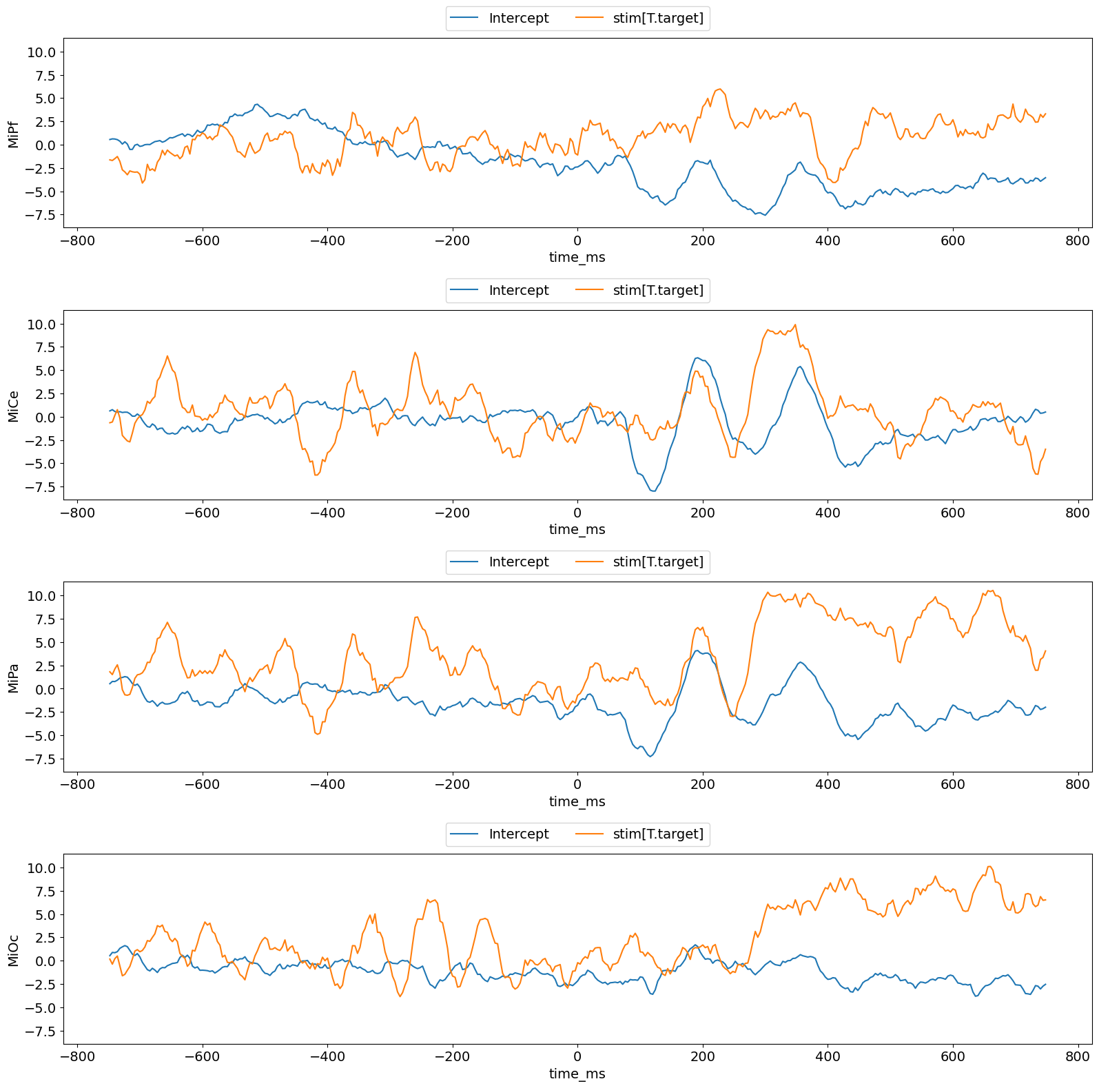
Plot results with a fitgrid built-in.

f, axs = lm_grid.plot_betas()
quickstart

Or make your own with pandas, matplotlib, seaborn, etc..

from matplotlib import pyplot as plt

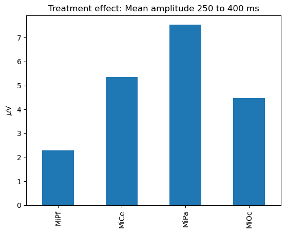
# Slice a time range and compute means with pandas
p3_effect = lm_grid.params.loc[
    pd.IndexSlice[250:400, "stim[T.target]"], :
].mean()

ax = p3_effect.plot.bar()
ax.set_title("Treatment effect: Mean amplitude 250 to 400 ms")
_ = ax.set(ylabel="$\mu$V")
Treatment effect: Mean amplitude 250 to 400 ms
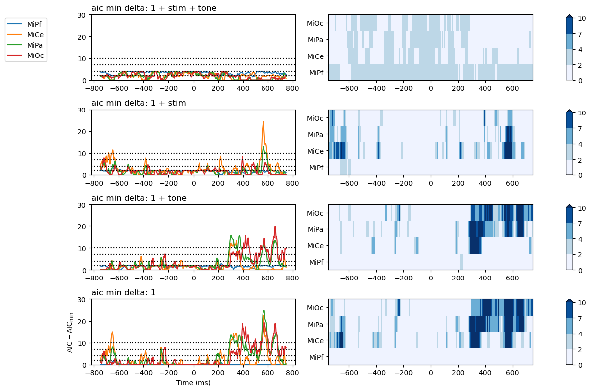
  1. Compare grid summaries for models sets and pairs.

from fitgrid.utils import summary as fgs

p3_summaries = fgs.summarize(
    p3_epochs_fg,
    modeler="lm",
    RHS=["1 + stim + tone", "1 + stim", "1 + tone", "1"],
    LHS=["MiPf", "MiCe", "MiPa", "MiOc"],
    quiet=True,
)
p3_summaries
MiPf MiCe MiPa MiOc
time_ms model beta key
-748 1 + stim + tone Intercept 2.5_ci -6.503946 -3.857680 -4.059197 -2.997439
97.5_ci 5.533294 1.591338 1.775272 1.376619
AIC 3380.292996 2850.856368 2896.512769 2704.067358
DF 331.000000 331.000000 331.000000 331.000000
Estimate -0.485326 -1.133171 -1.141962 -0.810410
... ... ... ... ... ... ... ...
748 1 Intercept SSresid 183325.213323 84402.889127 94649.943726 66876.807339
T-stat -2.344876 -0.072978 -1.444980 -1.913042
has_warning 0.000000 0.000000 0.000000 0.000000
logLike -1527.340759 -1397.805528 -1416.940998 -1358.936378
sigma2 550.526166 253.462130 284.234065 200.831253

36000 rows × 4 columns


Compare models on Akiake’s information criterion (AIC) as the difference between the model’s AIC and the lowest in the set. Larger AIC differences indicate relatively less support for the model in comparison with the alternative(s).

fig, axs = fgs.plot_AICmin_deltas(p3_summaries)
for axi in axs:
    axi[0].set(ylim=(0, 30))
axs[-1][0].set(xlabel="Time (ms)", ylabel="$\mathsf{AIC - AIC_{min}}$")
fig.tight_layout()
aic min delta: 1 + stim + tone, aic min delta: 1 + stim, aic min delta: 1 + tone, aic min delta: 1

Total running time of the script: ( 1 minutes 10.332 seconds)

Gallery generated by Sphinx-Gallery