User Guide
TL;DR These are notes and highlights. For usage see the Workflow Outline, Examples Gallery, and API
fitgrid Epochs
Fitting linear regression models in Python and R with formulas like
y ~ a + b + a:b in Python (patsy,
statsmodels.formula.api) or R (lm,
lme4::lmer) assumes the data are represented as a 2D array with the
variables in named columns, y, a, b and values
(“observations”, “scores”) in rows.
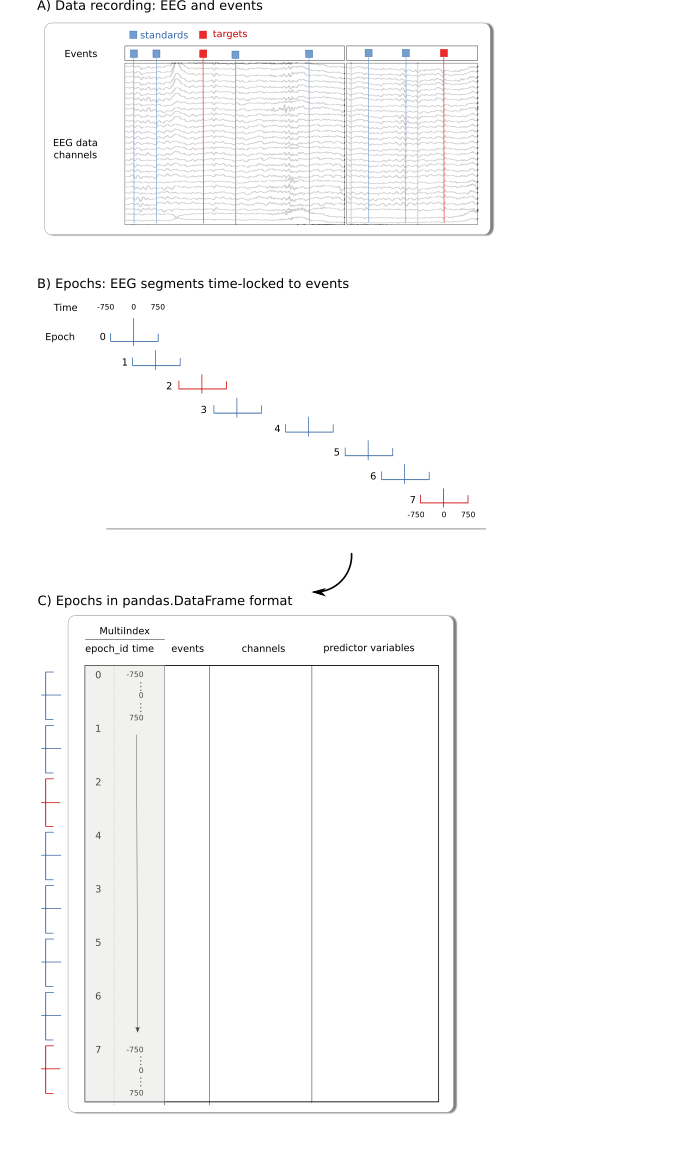
fitgrid follows this format with the additional assumption that
the data are vertically stacked fixed-length time-series “epochs”, so
the user must specify two additional row indexes that together
uniquely identify the epoch and timestamp of each data row.
Epochs data format
Data for fitgrid modeling should be prepared as a
single pandas.DataFrame with a
pandas.MultiIndex as follows:
- MultiIndex names and data types
Each epoch must have a unique integer identifier in the
epoch_idindex. The index values need not be ordered and gaps are allowed but duplicate epoch indices are not. Thetimeindex integer timestamps must be the same for all epochs. Gaps and irregular intervals between timestamps are allowed, duplicate timestamps within an epoch are not.epoch_id(default): integertime(default): integer
The MultiIndex names default to
epoch_idandtimebut any index column may be designated as the epoch or time index, provided the conditions are met. Event-relative epochs are often time-stamped so the event is at time=0 but this is not afitgridrequirement and the temporal resolution of the timeseries is not specified. For data epochs with time index values -10, 0, 10, 20, theFitGrid[-10:20, channels]object will be the same whether the timestamps denote milliseconds or months.- Data columns
channel data columns: numeric
predictor variable columns: numeric, string, boolean
- Example:
A canonical source of data epochs for
fitgridare multichannel “strip charts” as in EEG and MEG recordings. In this case, the epochs are regularly sampled fixed-length segments extracted from the strip chart and time-stamped relative to an experimental event.
Data Ingestion
Rows and columns epochs data can be loaded into a fitgrid
Epochs object from a
pandas.DataFrame in memory or read from files in feather or HDF5 format. For details
on using these data formats see pandas.read_feather() and and
pandas.read_hdf().
Data Simulation
fitgrid has a built-in method fitgrid.fake_data.generate() that
returns a Epochs data objects or
pandas.DataFrame for testing.
EEG Sample Data
Optional sample files containing previously prepared EEG data epochs are availble for download from the Zenodo archive at eeg-workshops/mkpy_data_examples/data.
The files can be installed into the fitgrid package with
fitgrid.sample_data.get_file() and accessed thereafter as
fitgrid.DATA_DIR(<filename>) or downloaded manually to another
location.
The sample data with msNNN.epochs.* filenames contain segmented EEG
epochs and the msNNNN infix gives the length of the epoch in
millesconds. Files with the shortest epochs (100 ms) are suitable for
testing, those with longer epochs (1500, 3000 ms) are more
representative of actual experimental EEG data. The feather format
versions *.epochs.feather are recommended for use with pandas
pandas.read_feather().
Additional information about the experimental designs for these sample files is available online at https://eeg-workshops.github.io/mkpy_data_examples.
Fitting a model
The following methods populate the FitGrid[times,channel] object with statsmodels results for OLS
model fits and lme4::lmer for linear mixed-effects fits.
Ordinary least squares:
fitgrid.lmlm_grid = fitgrid.lm( epochs_fg, RHS='1 + categorical + continuous' )
Linear mixed-effects:
fitgrid.lmerlmer_grid = fitgrid.lmer( epochs_fg, RHS='1 + continuous + (continuous | categorical)' )
User-defined (experimental):
fitgrid.run_model
The FitGrid[times, channels]
Slice by time, channel
Slice the FitGrid[times, channels]
with pandas.DataFrame range : and label slicers. The
range includes the upper bound.
lm_grid[:, ["MiCe", "MiPa"]]
lm_grid[-100:300, :]
lm_grid[0, "MiPa"]
Access results
Query the FitGrid[times, channels]
results like a single fit object. Result grids are returned as a
pandas.DataFrame or another FitGrid[times, channels] which can be queried the same way.
lmg_grid.params
lmg_grid.llf
Slice and access
lm_grid[-100:300, ["MiCe", "MiPa"].params
fitgrid.LMFitGrid() methods
The fitted OLS grid provides time-series plots of selected model
results: estimated coefficients fitgrid.lm.plot_betas() and
adjusted \(R^2\) fitgrid.lm.plot_adj_rsquared() (see also
fitgrid.utils() for additional model summary wrappers).
Saving and loading grids
Running models on large datasets can take a long time. fitgrid lets you save your grid to disk so you can restore them later without having to refit the models. However, saving and loading large grids may still be slow and generate very large files.
Suppose you run lmer like so:
grid = fitgrid.lmer(epochs, RHS='x + (x|a)')
Save the grid:
grid.save('lmer_results')
Later you can reload the grid:
grid = fitgrid.load_grid('lmer_results')
Warning
Fitted grids are saved and loaded with Python pickle which is not guaranteed to be portable across different versions of Python. Unpickling unknown files is not secure (for details see the Python docs). Only load grids you trust such as those you saved yourself. For reproducibility and portability fit the grid, collect the results you need, and export the dataframe to a standard data interchange format.
Model comparisons and summaries
To reduce memory demands when comparing sets of models, fitgrid
provides a convenience wrapper, fitgrid.utils.summarize, that
iteratively fits a list of models and collects a lightweight summary
dataframe with key results for model interpretation and
comparison. Unlike FitGrid[times, channels] objects, the summary dataframe format is the
same for fitgrid.lm and fitgrid.lmer. Some helper functions are
available for visualizing selected summary results.
Model and data diagnostics (WIP)
Model and data diagnostics in the fitgrid framework is work in progress. For ordinary least squares fitting, there is some support for the native statsmodels OLS diagnostic measures. Diagostics that can be computed analytically from a single model fit, e.g., via the hat matrix diagonal, may be useable but many are not for realistically large data sets. The per-observation diagnostic measures, e.g., the influence of observations on estimated parameters, are the same size as the original data multiplied by the number of model parameters which may overload memory and measures that require on leave-one-observation-out model refitting take intractably long for large data sets. A minimal effort is made to guard the user from known trouble but the general policy is fitgrid stays out of the way so you can try what you want. If it works great, if it chokes, that’s the nature of the beast you are modeling.
Support for linear-mixed effects diagnostics in fitgrid is limited to a variance inflation factor computation implemented in Python as a proof-of-concept. fitgrid does not interface with mixed-effect model diagnostics libraries in R and plans are to improve support for mixed-effects modeling in Python rather than expand further into the R ecosystem.
fitgrid under the hood
How mixed effects models are run
Mixed effects models do not have a complete implementation in Python, so we interface with R from Python and use lme4 in R. The results that you get when fitting mixed effects models in fitgrid are the same as if you used lme4 directly, because we use lme4 (indirectly).
Multicore model fitting
On a multicore machine, it may be possible to significantly speed
fitting by computing the models in parallel especially for
fitgrid.lmer. For least squares
models, fitgrid.lm uses statsmodels
under the hood, which in turn employs numpy for calculations.
numpy itself depends on linear algebra libraries that might be
configured to use multiple threads by default. This means that on a 48
core machine, common linear algebra calculations might use 24 cores
automatically, without any explicit parallelization. So when you
explicitly parallelize your calculations using Python processes (say 4
of them), each process might start 24 threads. In this situation, 96
CPU bound threads are wrestling each other for time on the 48 core
CPU. This is called oversubscription and results in slower
computations.
To deal with this when running fitgrid.lm, we try to instruct the linear algebra libraries
your numpy distribution depends on to only use a single
thread in every computation. This then lets you control the number of
CPU cores being used by setting the n_cores parameter in
fitgrid.lm and fitgrid.lmer.
If you are using your own 8-core laptop, you might want to use all but
one core, so set something like n_cores=7. On a shared machine,
it’s a good idea to run on half or 3/4 of the cores if no one else is
running heavy computations.
Note that fitgrid parallel processing counts the “logical” cores
available to the operating system and this may differ from the number
of physical cores, depending on the system hardware and setting, e.g.,
Intel CPUs with hyperthreading enabled. The Python package
psutil and
psutil.cpu_count(logical=True) and
psutil.cpu_count(logical=False) may be useful for interrogating
the system about the available resources.